The Rayleigh Quotient

Eigenvalue analysis wasn’t giving me what I wanted the other day. So, to make a long story short, I decided to try Rayleigh’s method.

I won’t go through all the details of Rayleigh’s method, but the basic idea is you can obtain a very good approximation of the fundamental frequency of a structural model by using the displacements due to a static analysis as the shape function in Rayleigh’s quotient.

This makes sense–the eigenvalue equation, , is one of static equilibrium.

After some manipulation (see Chapter 8 of the Chopra book, 5th ed.), Rayleigh’s quotient can be expressed as

where u_j is the displacement at the j^th degree-of-freedom (DOF) due to static loads in direct proportion to the mass at the DOF, i.e., a load pattern where F_j=m_j*g at each DOF in the direction of vibration.

Implementing Rayleigh’s method in OpenSees is pretty straightforward. I’ll show the method with Example 8.9, a five story shear frame from the Chopra book.

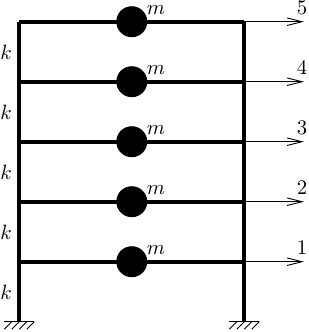
There’s a few ways to define shear frame models. My favorite approach is to use a one-dimensional model with zero length springs in series.

N = 5 # Number of stories
k = 110 # Story stiffness
m = 1.25 # Floor mass

g = 386.4

ops.wipe()
ops.model('basic','-ndm',1,'-ndf',1)

ops.uniaxialMaterial('Elastic',1,k)

ops.node(0,0); ops.fix(0,1)
for j in range(N):
    ops.node(j+1,0)
    ops.mass(j+1,m)
    ops.element('zeroLength',j+1,j,j+1,'-mat',1,'-dir',1)

The code to define a load pattern and compute the Rayleigh quotient is easy for the common case where mass is lumped at the nodes.

ops.timeSeries('Constant',1)
ops.pattern('Plain',1,1)
for j in range(N):
    mj = ops.nodeMass(j+1,1)
    ops.load(j+1,mj*g)
    
ops.analysis('Static')
ops.analyze(1)

num = 0; den = 0
for j in range(N):
    mj = ops.nodeMass(j+1,1)
    uj = ops.nodeDisp(j+1,1)
    num += mj*uj
    den += mj*uj*uj
    
w2 = g*num/den
print(f'Rayleigh: w2 = {w2}, Period = {2*3.14159/w2**0.5}')
w2 = ops.eigen(1)[0]
print(f'Eigenanalysis: w2 = {w2}, Period = {2*3.14159/w2**0.5}')

That’s right, I used 3.14159 for . If you’re not using numpy or math for anything else, there’s no need to import these packages and all their baggage just to get 16 digits of .

For models with more than one DOF per node, the code to compute the Rayleigh quotient is similar to what’s shown in this post on modal participation factors.

Here are the results for this simple model.

The period is pretty long for a five story frame; however, sometimes a number is a number.