ARPACK, the default eigenvalue solver in OpenSees, is very good at quickly finding a small number of eigenpairs (frequencies and mode shapes) for large models. Getting a few of a model’s lowest frequencies so you can check for rigid body modes and/or calculate Rayleigh damping coefficients is all most users care about. ARPACK gets the job done and you can move on to response history analysis by direct time integration.
However, ARPACK often struggles when you ask for many modes, especially in models with static DOFs, e.g., frame models with lumped translational mass. For such models, it’s not uncommon for ARPACK to return an error if you ask for several modes.
But, even for models without static DOFs, ARPACK can give unexpected results when applying modal damping or modal superposition to models with repeated, or degenerate, eigenvalues.
Consider a simple model of a two-story building with identical story stiffness, k=610 kip/inch, in two orthogonal directions, and masses m1=1 kip-s2/inch and m2=0.5 kip-s2/inch. The model has N=4 dynamic DOFs.

Without loss of generality in the forthcoming results, this model can be implemented in OpenSees using two zero length elements, each with elastic materials defined in two directions.
import openseespy.opensees as ops

# Units = kip, inch, sec

g = 386.4

k = 610
m1 = 1.0
m2 = 0.5

ops.wipe()
ops.model('basic','-ndm',2,'-ndf',2)

ops.node(0,0,0); ops.fix(0,1,1)
ops.node(1,0,0); ops.mass(1,m1,m1)
ops.node(2,0,0); ops.mass(2,m2,m2)

ops.uniaxialMaterial('Elastic',1,k)

ops.element('zeroLength',1,0,1,'-mat',1,1,'-dir',1,2)
ops.element('zeroLength',2,1,2,'-mat',1,1,'-dir',1,2)

ops.eigen(3)
OpenSees gives the following three eigenvalues:
[357.32972695241205, 357.32972695241205, 2082.670273047587]
The excruciatingly high number of significant figures shows the first two modes are indeed repeated. These values check out against hand calculations.
The corresponding eigenvectors may seem reasonable at first glance:
[[ 0.26070429  0.65729238 -0.60120583]
 [ 0.65729238 -0.26070429 -0.37222513]
 [ 0.36869155  0.9295518   0.85023344]
 [ 0.9295518  -0.36869155  0.52640583]]
Moving beyond casual inspection though, you’ll see that the mode shapes for the two orthogonal directions are coupled:
- Mode 1 is primarily first mode Y-direction vibration, close to the correct mode shape of [0,1/√2,0,1], but with some noise in the X-direction DOFs.
- Mode 2 is close to the correct mode shape, [1/√2,0,1,0], for first mode X-direction vibration, along with some noise in the Y-direction DOFs.
- Mode 3 is second mode X-direction vibration, [−1/√2,0,1,0], plus noise in the Y-direction DOFs.
On the upside, the eigenvectors are mass orthonormal, so the noise in the orthogonal directions is not random noise. Mass orthonormality is easily verified for models with lumped nodal mass.
import numpy as np

N = ops.systemSize()
Nmodes = N-1

Mn = [0]*Nmodes
for n in range(Nmodes):
    for nd in ops.getNodeTags():
        phi = np.array(ops.nodeEigenvector(nd,n+1))
        mass = np.diag(ops.nodeMass(nd))
        Mn[n] += phi.T@mass@phi
    assert np.isclose(Mn[n],1.0)
Despite the mass orthonormality, these coupled eigenvectors will affect ensuing analyses for modal properties, modal damping, and modal superposition. Although this model is simple, I’ve been burned by this eigenvector issue on more complex models for the following cases and wasted hours debugging up the wrong tree.
Modal Properties
With the coupled eigenvectors, the model’s mass participation is a bit stunted. The X-direction mass participation factors and cumulative percentage of participating mass are shown below.
| Mode | Participation (X-dir) | Cumulative |
|---|---|---|
| 1 | 0.44505 | 13.20% |
| 2 | 1.1221 | 97.14% |
| 3 | -0.17609 | 99.21% |
Both modes 1 and 2, the fundamental modes of vibration in the X and Y directions, respectively, contribute to the mass participation in the X-direction. The correct solution for X-direction mass participation is that mode 1 does not participate and mode 2 has 97.14% mass participation in and of itself.
For more complex models, the incorrect cumulative mass participation for models with degenerate eigenvalues can lead to interpretation errors or require more modes than necessary to reach a target participating mass.
Modal Damping
The coupling of eigenvector components in orthogonal directions can lead to strange results with modal damping. Consider an analysis of the simple spring model for constant (step) loading where 3% damping is used in each mode.
ops.modalDamping(0.03)

ops.timeSeries('Constant',1)
ops.pattern('Plain',1,1)
ops.load(1, 70,0)
ops.load(2,100,0)

Tfinal = 5
dt = 0.01
Nsteps = int(Tfinal/dt)

ops.analysis('Transient','-noWarnings')
ops.analyze(Nsteps,dt)
Although the forcing function is only in the X-direction, the model has non-zero response in the Y-direction due to modal damping forces generated from the “bad” eigenvectors.
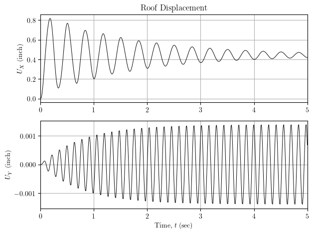
The magnitude of the Y-direction displacement is small relative to the X-direction displacement, but for more complex models, the “out of plane” response could be more significant.
I kept the forcing function simple so we could see the response clearly, but you’ll see the same behavior for earthquake excitation when using modal damping and the default eigenvalue solver on models with degenerate eigenvalues.
Modal Superposition
Although OpenSees computes dynamic response by direct time integration, you may be inclined to implement modal superposition at the script level as an exercise or to cross-check OpenSees against another software that is based on modal superposition.
Summing modal responses over N-1 modes for the simple spring model (with no damping) subjected to the same step loading as the previous demonstration gives the results shown below.
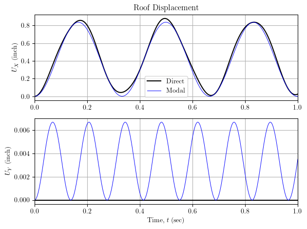
Like in the previous demonstration, we see spurious “out of plane” (Y-direction) displacement response due to the coupling terms in the eigenvectors. For direct integration, the Y-direction displacement is zero, as expected.
The X-direction displacement obtained by modal superposition is close to direct integration, but perhaps not as close as you would expect when including N-1 modes, especially for this model where the first three modes cover 99.21% of the participating X-direction mass.
If you implement modal superposition at the script level for more complex models with degenerate eigenvalues and with eigenvectors computed from the default eigenvalue solver, you may struggle to superimpose enough modes to get reasonably close to direct integration.
Don’t Worry Though
I have two closing statements.
First, no, Frank did not mess up. This is not an OpenSees issue, but rather a well-known ARPACK issue. You can re-create this analysis in Python and call the eigsh function, which is also a wrapper to the ARPACK library.
from scipy.sparse.linalg import eigsh

M = np.diag([m1,m1,m2,m2])

K = np.zeros((4,4))
K[0,0] = 2*k; K[0,2] = -k
K[2,0] =  -k; K[2,2] =  k
K[1,1] = 2*k; K[1,3] = -k
K[3,1] =  -k; K[3,3] =  k

lam,x = eigsh(K,M=M,k=3,which='SM')
For larger models, use the printA function to obtain the mass and stiffness matrices. For this model, eigsh will give the same eigenvalues as what’s reported from OpenSees:
[ 357.32972695 357.32972695 2082.67027305]
And the corresponding eigenvectors are a little different, but still mass orthonormal.
[[ 0.65729238 -0.26070429  0.37222513]
 [-0.26070429 -0.65729238 -0.60120583]
 [ 0.9295518  -0.36869155 -0.52640583]
 [-0.36869155 -0.9295518   0.85023344]]
Second, this is a case where not having a perfectly symmetric model is a good thing. The lack of symmetry will hide the ARPACK solver’s issue with degenerate eigenvalues. The odds are pretty high that your 3D models are not perfectly symmetric (even if you thought they were) and you will continue to be safely unaware of this issue in your IDAs with modal damping. Even a difference in the sixth significant figure of a stiffness or mass coefficient–one fiber of hair slightly askew on your model’s head–is enough to make the model numerically asymmetric.
Although the foregoing analyses were based on a simple model, you should be on the lookout for odd modal responses in 3D models of buildings with symmetric plan and no mass eccentricity, and possibly in 3D models of shafts, pipes, beams, etc. with doubly symmetric cross sections.
But generally, you can breathe a sigh of relief.
It’s easy to overlook “Almost Hear You Sigh” among many hits from the Rolling Stones.
Keith Richards has that stone cold look in his eyes.

[celebrate] JS Nie reacted to your message:
LikeLike