Murum, cura te ipsum

OpenSees has its fair share of element implementations that are computationally inefficient. Fortunately, most of those elements are never used.

But among elements that are used, SFI-MVLEM is the undisputed champion.

Whereas the standard MVLEM element uses a uniaxial material in each fiber, the SFI-MVLEM element accounts for the interaction of axial and shear stress ( and ) in each fiber using a plane stress NDMaterial. The only challenge is the normal stress, , must be zeroed out in each fiber.

To enforce =0 in each fiber, the element adds a node to the domain–one node for each fiber. Each node has only one DOF and its resisting force is proportional to the fiber’s  stress. So, if the global solution reaches zero residual, each fiber will be in a state of zero normal stress. Makes sense. It works.

But letting the global solution zero out fiber stresses is like throwing your garbage out on the street then admiring your clean home.

And, like throwing your garbage out on the street, those additional nodes cause huge global problems.

Consider the minimal shear wall example from a previous post. A 3D model is shown, but the issues apply to 2D models as well.

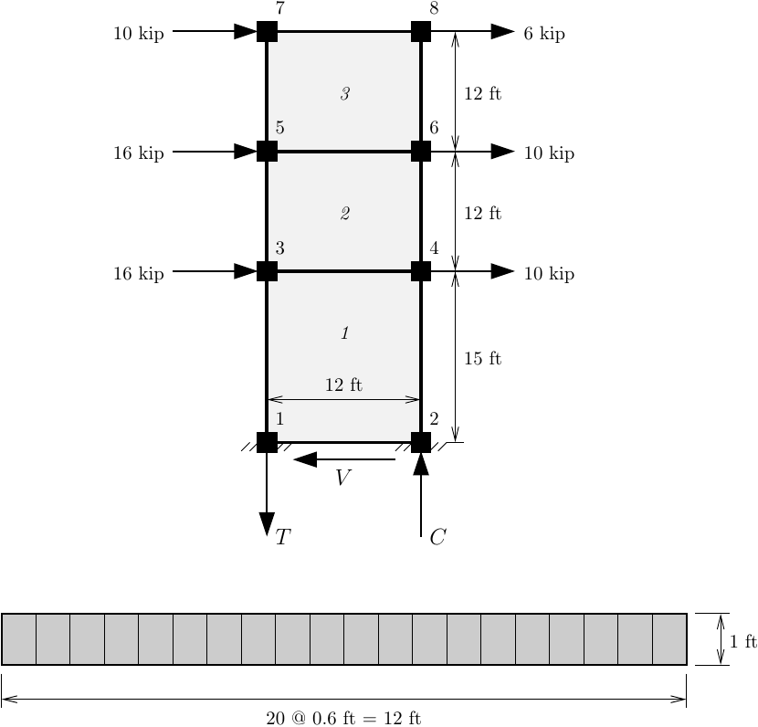
The definition of nodes and loads is identical to the previous post; the only difference is the material and element definition. Here an elastic-isotropic material is used, so the analysis should be simple.

N = 20 # Fibers

Ec = 3600*ksi
nu = 0.25
b = 1*ft
h = 12*ft

ops.nDMaterial('ElasticIsotropic',1,Ec,nu)

conc = [1]*N
bList = [b]*N
hList = [h/N]*N
ops.element('SFI_MVLEM',1,1,2,4,3,N,0.4,'-thick',*bList,'-width',*hList,'-mat',*conc,'-Eave',Ec)
ops.element('SFI_MVLEM',2,3,4,6,5,N,0.4,'-thick',*bList,'-width',*hList,'-mat',*conc,'-Eave',Ec)
ops.element('SFI_MVLEM',3,5,6,8,7,N,0.4,'-thick',*bList,'-width',*hList,'-mat',*conc,'-Eave',Ec)

Four obvious problems with the SFI-MVLEM element implementation are described below. But I didn’t write this post to point out problems and not offer solutions–that would be complaining, not writing–so, a mitigation strategy is offered for each issue.

1. Inconsistent Tangent

The first thing you will notice when running the minimal wall example with SFI-MVLEM elements is the excessive number of iterations. Remember, the wall constitutive model is linear-elastic, so equilibrium should be found in one iteration. But the analysis takes 18 iterations with the Newton-Raphson algorithm.

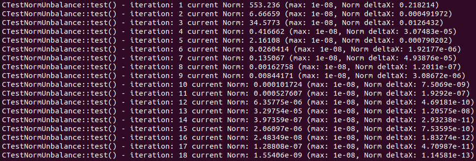
The slow convergence for linear response indicates an inconsistent tangent coming from the element. I haven’t confirmed the source of the inconsistent tangent, but I suspect the separation of the 22 from the 11 and 12 terms in the fiber tangent is not handled properly. There needs to be some static condensation, akin to what happens in the BeamFiber2dPS wrapper class, but I don’t see that happening in the SFI-MVLEM source code. Making matters worse, it appears the SFI-MVLEM ignores the tangent terms that couple axial and shear stresses in each fiber.

Mitigation

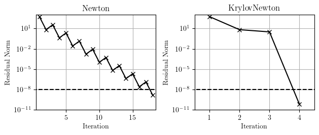
The Krylov-Newton algorithm can be effective at dealing with sloppy tangents. For this minimal wall example, the Krylov-Newton algorithm requires only four iterations.

OK, this issue has nothing to do with the additional internal nodes. But, as shown in the next two issues, those additional nodes make for more equations, and more equations translates to longer solve times. So, if you have to sit through more iterations because of an inconsistent tangent, you will notice longer run times, particularly for large models.

2. System Size

Using standard MVLEM elements for this simple wall model, the system size is 42 equations, but with the SFI-MVLEM elements, the system size is 102 equations. The resulting topologies of the stiffness matrix are shown below (using Plain numberer).

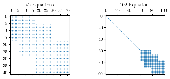
Both matrices have the same bandwidth (about 25), but due to the additional equations, the SFI-MVLEM model will have longer solve times, especially if you use a solver that assumes banded matrix storage or, even worse, full matrix storage. And the number of equations and solve time only go up if you increase the number of fibers in each SFI-MVLEM element.

Mitigation

If you must use SFI-MVLEM elements, use as few fibers as possible.

3. Equation Numbering

Compounding the longer solve times, the default equation numberer, RCM, and the lesser used AMD, can produce larger matrix bandwidths than the Plain numberer. The equation numbering algorithms deal with the extra SFI-MVLEM nodes in their own ways.

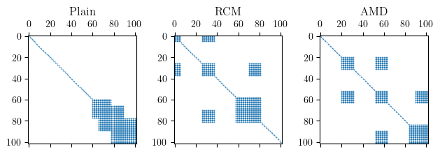
This may be the only case where using RCM is significantly worse than the Plain numberer. But for larger models, you’ll probably be better off sticking wtih RCM for the equation numbering.

Mitigation

Use a linear equation solver with sparse matrix storage, e.g., UmfPack, SparseGeneral, or Mumps. With sparse matrix storage, the topology of the stiffness matrix and the equation numbering don’t matter much, only the number of non-zero matrix entries.

4. Internal Node Tags

Although the model has eight user-defined nodes, if you print out the list of node tags (using ops.getNodeTags()), you will see there are 68 nodes defined in the domain–the eight nodes plus 60 nodes, one for each of the 20 fibers in each of the three elements.

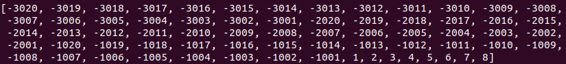
For each element, the internal node tags range from -(1000*eleTag+1) to -(1000*eleTag+Nfibers), e.g., element 2 creates nodes with tags -2001 to -2020.

Mitigation

There’s no getting around this implementation decision. Avoid defining nodes with negative tags–something that OpenSees allows. Similarly, don’t define SFI-MVLEM elements with negative tags as this could lead to collisions with positive node tags defined elsewhere in your model.

Conclusions

Using the default analysis options in OpenSees, you can experience unnecessarily long run-times in the analysis of SFI-MVLEM models. If you have to stick with the SFI-MVLEM elements, remember the following:

• Use as few fibers as possible
• Use a sparse matrix solver like UmfPack or Mumps
• Use the Krylov-Newton algorithm
• Be careful using negative node tags elsewhere in your model

If you have some latitude, take a small step over to the E-SFI-MVLEM element, which is the cura te ipsum for SFI-MVLEM. The element imposes an empirically derived shape function on the  strain field so that the problematic internal nodes are not necessary. The “E” at the front of E-SFI-MVLEM stands for “Efficient”, which is not an inaccurate description, but some minor issues remain.