Just Fillin’ Up the Tank

You’re not going to conquer incremental dynamic analysis of 3D reinforced concrete frame models the first day you use OpenSees. Some try, but they all fail. Those who start with simple test cases and level up in complexity will succeed.

The same goes for fluid-structure interaction. You will not conquer tsunami loading on structures the first day you use the particle finite element method (PFEM) in OpenSees. You have to start small.

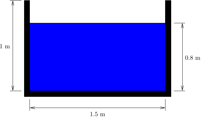
So, let’s start with a simple numerical wave tank (NWT) and verify some basic hydrostatic responses. The tank is 1.5 m long and 0.5 m wide with 1 m high walls. The standing water level is 0.8 m. The features and dimensions of this NWT can easily be changed for more complex simulations.

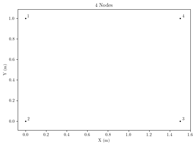
In OpenSees, the tank walls and floor are defined with regular nodes, beginning with the corner points.

import openseespy.opensees as ops

ops.wipe()
ops.model('basic','-ndm',2,'-ndf',2)

kg = 1
m = 1
sec = 1

N = kg*m/sec**2
Pa = N/m**2

g = 9.81*m/sec**2

Ltank = 1.5*m
Htank = 1*m
hfluid = 0.8*m
tfluid = 0.5*m

ops.node(1,0,Htank)
ops.node(2,0,0)
ops.node(3,Ltank,0)
ops.node(4,Ltank,Htank)

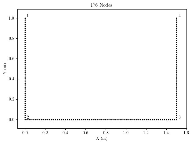
Then, more nodes, each with two DOFs, are created between the corner nodes using the line mesh command. The nodes of the tank walls are considered structure nodes for FSI computations. All nodes on the tank boundary are fixed against motion. These intermediate nodes are required along the tank walls and floor so that fluid does not leak out when the tank is filled.

meshsize = 0.02*m

# Create tank walls and floor
sid = 1
walltag = 1
ops.mesh('line', walltag, 4, *[1,2,3,4], sid, 3, meshsize)

wallnodes = ops.getNodeTags('-mesh', walltag)
for nd in wallnodes:
    ops.fix(nd, 1, 1, 1)

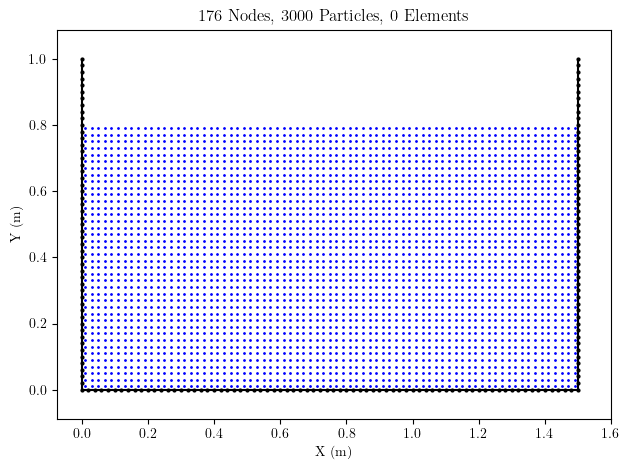
The fluid particles are created next using the particle mesh command. The number of particles in the X and Y directions is based on the tank dimensions and the mesh size. For hydrodynamic simulations, we’d want to use more particles by setting numx and numy to 2 or higher.

# Fluid properties
rho = 1000*kg/m**3 # density
mu = 1e-3*kg*m/sec # viscosity
kappa = -1.0 # incompressible flow

# Number of particles per cell
numx = 1.0
numy = 1.0

nx = int(round(Ltank/meshsize)*numx)
ny = int(round(hfluid/meshsize)*numy)

# Create fluid particles and element arguments for meshing
eleArgs = ['PFEMElementBubble', rho, mu, 0, -g, tfluid, kappa]
partArgs = ['quad', 0.0, 0.0, Ltank, 0.0, Ltank, hfluid, 0.0, hfluid, nx, ny]
parttag = 2
ops.mesh('part', parttag, *partArgs, *eleArgs)

The fluid particles created by the particle mesh command are shown below. The arguments for the fluid elements (PFEMElementBubble) are stored with the particle mesh, but will not be instantiated until the background mesh is created in the next step.

The background mesh command creates nodes and elements for the fluid mesh. For 2D models, the command requires lower left and upper right corners of a bounding box over which the background mesh should be created. The wall nodes are identified as structural rather than fluid nodes.

lower = [0,0]
upper = [Ltank, hfluid]
ops.mesh('bg', meshsize, *lower, *upper,
     '-structure', sid, len(wallnodes), *wallnodes)

Additional details on the background mesh formulation in OpenSees are described in Zhu and Scott (2022).

The element mesh is shown below (particles not shown). Note that two nodes are added for each location in the background mesh–one node to track motion (two DOFs) and one for a pressure constraint (one DOF). Thus, the total nodes in the domain is 6272 instead of 3224.

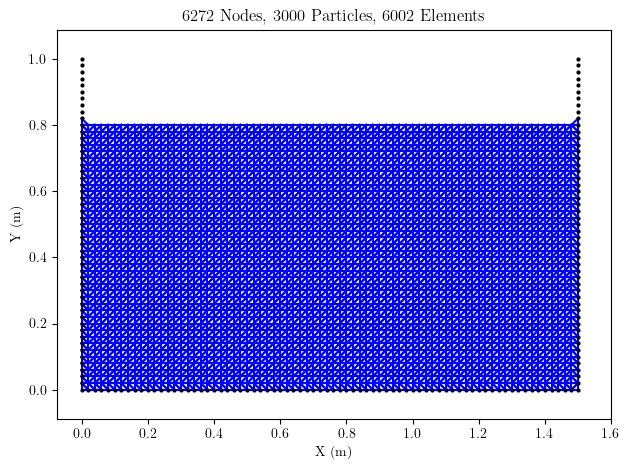
Note that the meshing creates an extra element between each tank wall and the fluid free surface. For hydrodynamic applications, the extra elements are not a big deal, but they are enough to throw off the forthcoming hydrostatic sanity checks. So, the two extra elements will be removed. If you follow the model creation above, you can remove elements with tags 5775 and 6002, e.g., ops.remove('element',5775).

With the nodes and elements of the tank defined, the analysis can begin. Just like a regular OpenSees analysis, you have to define each component of the analysis.

ops.constraints('Plain')
ops.numberer('RCM')
ops.test('PFEM', 1e-12, 1e-12, 1e-12, 1e-12, 1e-12, 1e-12, 10, 3, 1, 2)
ops.algorithm('KrylovNewton')
ops.integrator('PFEM', 0.5, 0.25)
ops.system('PFEM')

ops.analysis('PFEM', 5e-3, 1e-3, -g)
ops.analyze()

ops.reactions('-dynamic')

A few things to note about the analysis options:

• test – The PFEM convergence test uses relative and absolute tolerances on velocity and pressure (documentation). I’m using very small tolerances because the simulation is hydrostatic. For hydrodynamic simulations, you can get away with 1e-5.
• integrator – The PFEM integrator is Newmark with velocity as the primary unknowns.
• system – The PFEM system of equations is solved using UmfPack (documentation)
• analysis – In the PFEM analysis command, you specify the maximum and minimum time step and body force to apply to particles that separate from a mesh (documentation). Because this simulation is hyrdrostatic, the time step and particle separation are not terribly important.
• analyze – The PFEM analyze command always advances one, and only one, time step. So there is no number of time steps specified with this command.
• reactions – After the analysis, use the -dynamic option to include fluid element inertia in the assembly of reaction forces

The plot below shows the pressure at each node. I went bespoke with the vridis color map in a matplotlib scatter plot. Instead of wasting your time on unconventional color schemes that only you think look good, you should use ParaView, like in the videos linked to in this post. I also used a small mesh size to get smooth results for plotting. Again, you should use ParaView and a coarser mesh for this simulation.

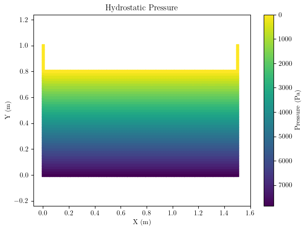
The pressure increases with fluid depth and is 7898 Pa at the bottom of the tank, matching the known solution of .

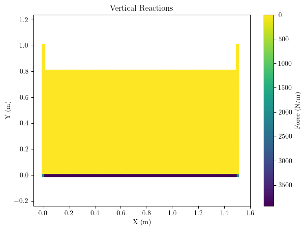
Vertical reactions are developed along the tank floor. The total vertical reaction matches the weight of the fluid, .

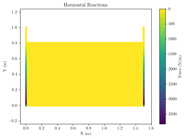
The horizontal reactions on the tank walls shown below increase with fluid depth. The intensity of the horizontal reactions increases from zero to .

There’s not much else to check here. Future posts will make minor tweaks to the NWT and the PFEM model and analysis for hydrodynamics and fluid-structure interaction.