P-M Interaction by the Book

Find any indeterminate beam, frame, or truss problem from a structural analysis textbook, and you can make OpenSees solve it. But sometimes, replicating the basics is not so easy. Take, for instance, an axial-moment (P-M) interaction diagram of reinforced concrete (RC) sections.

The typical approach advocated with OpenSees is to use repeated moment-curvature analyses over a range of axial loads. For each axial load applied on a zero length section, use displacement control with a reference moment–or proportional reference moments for biaxial bending–until reaching a target fiber strain, section curvature, or some other limit state.

However, this approach doesn’t match the textbook strain compatibility method for finding the strength of RC sections:

1. Assume the extreme concrete compression fiber is at 0.003 strain
2. Obtain a linear strain profile by assuming a neutral axis depth or a reinforcing steel strain
3. Compute stresses in the Whitney stress block (WSB) and the steel bars
4. Compute stress resultants from the WSB and steel bars
5. Determine the equivalent force-couple system acting at the section centroid

Repeat these steps over a range of neutral axis depths (or reinforcing steel strains) and you will generate a P-M interaction diagram. These steps are easily coded in MATLAB, Python, and even Excel.

The first point of this post is that we can make OpenSees do exactly this textbook WSB procedure. As usual, define your concrete and steel materials, put them in a fiber section, and then put that section in a zero length section element. Here we use Concrete01 which reaches its peak compressive strength, , at 0.002 strain and spalls at 0.006 strain. The steel is EPP.

ops.node(1,0.0,0.0)
ops.node(2,0.0,0.0)

ops.fix(1,1,1,1)
ops.fix(2,0,1,0)

fc = 4.0 # ksi
fy = 60.0 # ksi
E = 29000.0 # ksi

ops.uniaxialMaterial('Concrete01',concreteTag,fc,0.002,0,0.006)
ops.uniaxialMaterial('Steel01',steelTag,fy,E,0.0)

#
# Define your section (secTag)
#

ops.element('zeroLengthSection',1,1,2,secTag)

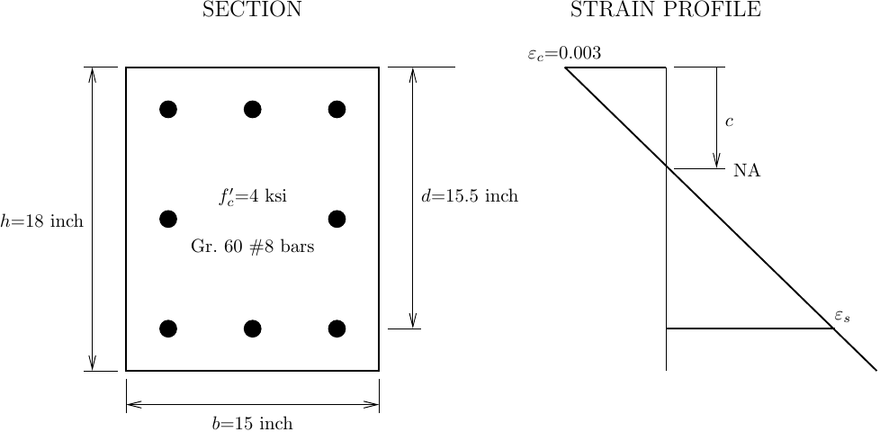
Then, for any strain in the “bottom” reinforcing steel, compute the strain profile. For reference, a rectangular RC section is shown below along with a strain profile.

Using the strain profile, we can use sp (single point) constraints to impose the axial deformation and curvature at the section centroid.

# e.g., at the balance point
epss = fy/E # Tension steel yield strain
kappa = (epss+epsc)/d
c = epsc/kappa # Depth to NA

ops.timeSeries('Constant',2)
ops.pattern('Plain',2,2)
ops.sp(2,1,-epsc + kappa*h/2) # Strain at the centroid
ops.sp(2,3,kappa) # Curvature

The axial load and bending moment are then the “reactions” on the node with the imposed sp constraints. Be sure to use 'Transformation' constraint handler and also use the 'UmfPack' solver as it’s the only solver that won’t rain on your parade for having all DOFs constrained.

ops.constraints('Transformation')
ops.system('UmfPack')

ops.analysis('Static')
ops.analyze(1)

ops.reactions()

P = -ops.nodeReaction(2,1)
M = ops.nodeReaction(2,3)

Put all of this in a loop over the steel strain, epss, from -0.003 (pure compression) to something large (say five times the steel yield strain) and you’ll get the P-M interaction curve shown below along with a straight-up Python implementation of the textbook WSB procedure.

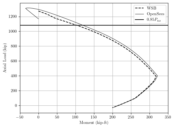
I’m not too worried about the OpenSees interaction curve taking a circuitous route to pure compression. The top of the interaction curve will get chopped off at 85% anyway due to “accidental moments”, the rumored sequel to a 2007 Judd Apatow movie. If you’re curious, the roundabout path is due to the descending branch of Concrete01 from 0.002 to 0.003 compressive strain. Use Concrete23 and you’ll see a different detour to pure compression.

However, there’s still a difference between the WSB approach and OpenSees for axial loads below 85% of the pure compression load.

So, the second point of this post is that we can make OpenSees match the textbook WSB approach. To this end, we need a concrete stress-strain model that has compressive stress equal to for compressive strains exceeding . This strain is based on similar triangles with the depth, , of the WSB, where is the WSB parameter which depends on .

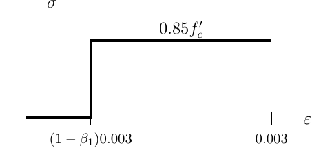
Nothing fits the bill, at least not directly. I can think of a couple kludgy workarounds, the least complicated of which is the ElasticMultiLinear material where we can define points that characterize the stress block.

fc = 4.0 # ksi
epsc = 0.003
beta1 = 0.85 # for 4 ksi concrete, smaller for higher strength concrete

strain = [-epsc,-epsc*(1-beta1),-epsc*(1-beta1),0]
stress = [-0.85*fc,-0.85*fc,0,0]
ops.uniaxialMaterial('ElasticMultiLinear',concreteTag,'-strain',*strain,'-stress',*stress)

Sure, with these inputs, the tangent of this material model is either zero of infinity, so I don’t recommend you use this model for general FEA. But this model is OK for our zero length section analysis because we’re not solving any nodal equilibrium equations–just imposing displacements and calculating forces.

As shown below, faking the WSB with ElasticMultiLinear instead of using Concrete01 gives a P-M interaction curve that agrees much better with the straight-up Python implementation of the WSB.

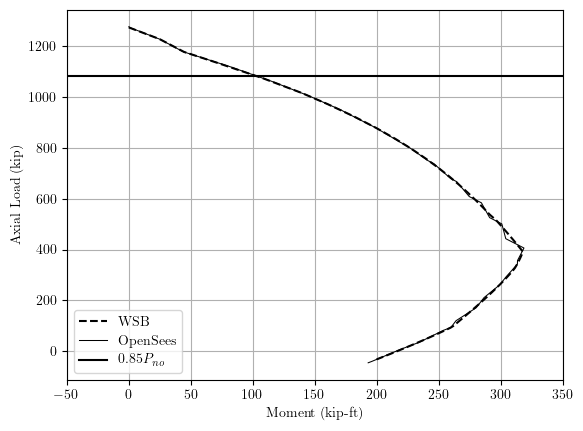
Due to the concrete fiber discretization, the OpenSees solution wiggles around the balance point (I used 20 fibers). These wiggles go away as you use more concrete fibers. Try it out yourself!

You read this far, so let’s see if you paid attention. How many unique factors of 0.85 does this post contain? Explain your response and the different 0.85 factors in the comments section below.