
Most beam-column elements in OpenSees take mass density, 

The elasticBeamColumn element can also return a consistent mass matrix with the -cMass input option.
ops.element('elasticBeamColumn',tag,...,'-mass',rho,'-cMass')
The dispBeamColumn and forceBeamColumn elements take the -cMass option as well, but the consistent mass is based on element-level mass density when the mass should be integrated from section mass density and shape functions. That’s a subject for another day, so this post will focus on the elasticBeamColumn element.
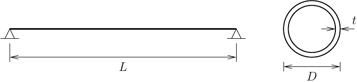
Consider a simply-supported steel pipe. The fundamental frequency (Hz) considering distributed mass density is 
For the analysis I’m going to show, you can choose whatever
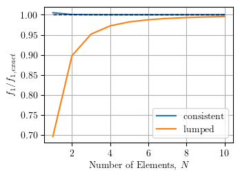
Discretizing the pipe into multiple elements, the fundamental frequency of the model should converge to the exact solution as the number of elements increases and the discrete masses approach distributed mass. Furthermore, using consistent element mass should give a better approximation than lumped element mass.

Both element mass formulations (lumped and consistent) give very good approximations (within 1%) for two elements and converge to the exact solution as more elements are used. Note that for one element, there are no dynamic DOFs with lumped mass. And with one element, the consistent mass approach gives a ratio of computed to exact frequency of 1.11.
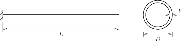
Now, let’s change the boundary conditions on the pipe from simple supports to cantilever. In this case, the fundamental period of vibration is 
Repeating the eigenvalue analysis for increasing number of elements and comparing lumped and consistent element mass, we get the results shown below.
Although both approaches converge to the exact solution, the consistent mass approach converges more quickly. The error for the lumped mass approach reduces to less than 5% when using three or more elements.

Hi Prof. Scott,
I had a question about recreating the results above for the cantilever beam. Below is the exact code I ran (I promise it’s not meant to be a debugging session) and I was able to get an exact frequency of ~12Hz for a beam with D = 10 and t = 1 with L = 100 for a steel member.
The problem is that as the number of elements increased, the frequency continued to decrease exponentially. It seems to be converging but I think it’s reaching a natural frequency of 0Hz. Wondering if there’s any reason why as the number of elements increase, the natural frequency would become lower.
import openseespy.opensees as ops
from math import pi as pi
import matplotlib.pyplot as plt
Set Model parameters
E = 2 * 106 # N/mm
R_out = 5 # mm
R_in = 4 # mm
I = pi/4*(R_out4 – R_in4) # mm^4
L = 100 #mm
A = pi*(R_out2 – R_in2) # mm^2
rho = 7.85 * 10-3 # g/mm^3
Calculated Exact
f1 = (3.5156/pi) / (2*L2) * (E*I/rho)0.5
print(f”Exact: {freq1_exact:.3f} Hz”)
print(“—-“)
data = []
Define the segments
for num_segments in range(2,50,2):
# Starts Analysis
ops.wipe()
ops.model(‘basic’,’-ndm’,2,’-ndf’,3)
ops.node(1,0,0)
ops.fix(1,1,1,1) # Fixes it
ops.geomTransf(‘Linear’,1)
for ii in range(1, num_segments+1):
ops.node((ii + 1), L * ii/(num_segments),0);
ops.element(‘elasticBeamColumn’, ii, ii, (ii+1), A,E,I,1,’-mass’,rho * A)
plt.plot(data,’-o’)
LikeLike
The eigenvalue solver you’re using only operates on K, not M and K: https://portwooddigital.com/2020/11/13/ordinary-eigenvalues/
Also, please read this post: https://portwooddigital.com/2023/02/12/not-everything-should-be-a-direct-translation/
LikeLike