Why Your Eigenvalue Analysis Failed

Eigenvalue analysis is often a necessary step before starting a dynamic response history analysis in OpenSees. You may want natural frequencies in order to compute Rayleigh damping coefficients, to apply modal damping, to compute modal properties, or to perform a response spectrum or modal superposition analysis.

However, eigenvalue analysis can fail, indicating a problem with your model but offering little insight into what went wrong. And even if you do use eigenvalue analysis to check your model, you still may wonder what the error message is telling you about the problem.

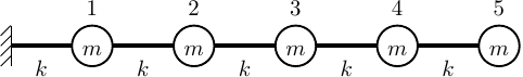
This post describes scenarios where an OpenSees eigenvalue analysis either fails or gives unexpected results. The scenarios are based on using OpenSees’s default eigenvalue solver, ARPACK, on a simple one-dimensional spring system with five dynamic DOFs, i.e., DOFs with mass.

The script for this model is shown below:

import openseespy.opensees as ops

k = 610
m = 1

N = 5 # Dynamic DOFs
Nmodes = 4 # Requested modes, N-1

ops.wipe()
ops.model('basic','-ndm',1,'-ndf',1)

ops.uniaxialMaterial('Elastic',1,k)

ops.node(0,0)
ops.fix(0,1)
for i in range(1,N+1):
    ops.node(i,0)
    ops.mass(i,m)
    ops.element('zeroLength',i,i-1,i,'-mat',1,'-dir',1)

w2 = ops.eigen(Nmodes)    

Using more complex frame or solid models would obscure whether failure of the eigenvalue analysis is due to modeling errors or element formulations of stiffness or mass. The eigenvalue solver does not care where the mass and stiffness come from, so a simple model is best to demonstrate failures.

As a reminder, the eigenvalue system of equations is assembled from stiffness and mass over the elements and nodes of your model.

The ARPACK eigenvalue solver uses the Lanczos algorithm to solve for the requested number of modes, or eigenpairs, $latex(\omega^2, {\bf x})$. The details of the Lanczos algorithm are not important here; however, the errors returned by ARPACK indicate how your model is ill-posed.

Dynamic DOFs

First, note that the ARPACK solver in OpenSees can compute eigenpairs for up to N-1 modes, where N is the number of dynamic DOFs. For this model with five dynamic DOFs, the four eigenvalues returned by the solver are as follows:

[49.4185721903132, 421.0699045867522, 1046.3758973065922, 1726.8063158623015]

If you ask for N modes on this or any properly defined model, you will receive the following error message:

ArpackSolver::Error with _saupd info = -3
NCV must be greater than NEV and less than or equal to N.
WARNING DirectIntegrationAnalysis::eigen() - EigenSOE failed in solve()

The wording about the size of NCV and NEV is a little cryptic, but basically it means you’re asking for too many modes.

As we’ll see later in this post, the phrase “up to N-1 modes” is important when your model has a mix of static (massless) and dynamic DOFs. But first, let’s go through some common modeling issues that cause an eigenvalue analysis to fail when all DOFs in your model are dynamic.

Singular Stiffness Matrix

A model with a singular stiffness matrix, e.g., due to insufficient boundary conditions or a rigid body mechanism, will have at least one eigenvalue equal to zero. Numerically, the eigenvalue solver will fail.

If we did not restrain the simple model against rigid body motion, e.g., by forgetting to fix node 0, we would see the linear equation solver fail and then the eigenvalue solver return an error.

ProfileSPDLinDirectSolver::solve() -  aii < 0 (i, aii): (5, 0)
ArpackSolver::Error with _saupd info = -9999
Could not build an Arnoldi factorization.
IPARAM(5) - the size of the current Arnoldi factorization is 5.
The user is advised to check that enough workspace and array storage have been allocated.
WARNING DirectIntegrationAnalysis::eigen() - EigenSOE failed in solve()

The output message Could not build an Arnoldi factorization indicates the eigenvalue analysis cannot proceed because the left-hand side matrix could not be factorized, bringing the Lanczos algorithm to a halt.

No Mass Matrix

Let’s suppose our model is properly restrained against rigid body motion and the response is fine for static analysis, but we forgot to define mass before attempting an eigenvalue analysis. In other words, the mass matrix is zero.

ArpackSolver::Error with _saupd info = -9
Starting vector is zero.
WARNING DirectIntegrationAnalysis::eigen() - EigenSOE failed in solve()

The output message Starting vector is zero means the solver cannot start the Lanczos algorithm because there is no mass on the right-hand side of the eigenvalue system of equations, i.e., no forcing function because the problem is ill-posed.

Indefinite Mass Matrix

A common modeling mistake is to define mass as a negative number. This error is easy to realize by defining a gravity load as negative–you know, because the load acts downward–then dividing that gravity load by the gravitational constant, g, and finally passing the resulting value to the mass command.

# Don't do this!
P = -100 # kip, downward
g = 386.4 # in/s^2
m = P/g
ops.mass(1,m,m,0)

We can demonstrate the outcome of a negative mass on our simple spring model by defining the mass at node 2 as negative, leading to an indefinite mass matrix. The error message from the eigenvalue solver is easy to miss and the solver will return numerical values for the eigenvalues.

ArpackSolver::Maximum number of iteration reached.
[6.92254474849224e-310, 6.92254474849224e-310, 6.92252241022947e-310, 4.8777955e-317]

With an indefinite mass matrix, the Lanczos algorithm does not converge and we see the message Maximum number of iterations reached with the returned eigenvalues all numerically zero.

Indefinite Stiffness Matrix

It’s also possible to have an indefinite stiffness matrix, which could be a sign of incorrect element parameters.

For our simple spring model, we can define the stiffness of spring 2 as negative, leading to an indefinite stiffness matrix. Unlike the case of negative mass, no error message is generated by the eigenvalue solver, but the “lowest” eigenvalue is now negative, which becomes problematic when you later take a square root looking for circular frequency and natural period.

[-727.3587559696524, 107.64756298256604, 452.0104739901504, 1159.4347304952619]

Physically, the negative eigenvalue means the model has modes of deformation that do not generate any resisting force. The other positive eigenvalues computed by the solver are not meaningful for the model.

Mixing Static and Dynamic DOFs

The last case replicates the most common error OpenSees users face when computing eigenvalues of frame models with lumped mass. The default eigenvalue solver struggles with the indefinite mass matrix that results from mixing dynamic translational DOFs with static (massless) rotational DOFs.

For our simple model, we can mimic this common problem with frame models by replacing each spring of stiffness k with two springs, each of stiffness 2k, connected in series. This configuration produces the same static response as the original model but mixes five static DOFs in with the dynamic DOFs.

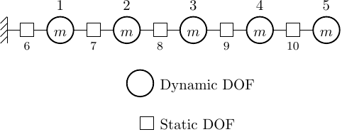
For this model, if we ask for only three modes, the eigenvalue solver will fail. In other words, two modes is all we can get out of this model with mixed DOFs. The massless DOFs render the mass matrix rank-deficient, reducing the number of eigenpairs the ARPACK solver can compute.

ArpackSolver::Error with _saupd info = -9999
Could not build an Arnoldi factorization.
IPARAM(5) - the size of the current Arnoldi factorization is 5.
The user is advised to check that enough workspace and array storage have been allocated.
WARNING DirectIntegrationAnalysis::eigen() - EigenSOE failed in solve()

There’s no general rule for how many eigenpairs can be successfully computed for a model with mixed DOFs. I’ve found that roughly half of the available modes can be computed, but the exact number is model dependent. The ratio of static to dynamic DOFs and the DOF numbering are possible factors in how many modes can be computed. For frame and shell models, using consistent element mass will reduce your number of static DOFs and allow you to compute additional modes for your model.

Summary

Below is a table summarizing the common errors, likely causes, and solutions for a failed eigenvalue analysis in OpenSees.

Although one might blame the solver in the case of mixed DOFs, eigenvalue analysis fails in all of these examples because the problem is ill-posed.

This post does not address multi-point constraints or the effect of constraint handlers on eigenvalue analysis. Constraint handlers in OpenSees modify the assembled mass and stiffness matrices, introducing issues that are beyond the basic model checks covered here.

This post also does not cover changes in eigenvalues during a nonlinear dynamic response history analysis where a model can become unstable and produce a negative eigenvalue after buckling or loss of load carrying capacity. Interpreting eigenvalues in this case is beyond the scope of this post.