Minimal DDM Examples

Although it was the subject of my first journal article and has been a welcome diversion since, other than one post, the direct differentiation method (DDM) has not seen much action on the blog.

With the DDM, you can compute accurate and efficient derivatives of the structural response with respect to various model and load parameters. The cruxes of the DDM are its derivation and its implementation; however, the OpenSees framework supports DDM implementations. But once you get over the derivation, the DDM makes structural reliability and optimization algorithms run much more quickly compared to computing derivatives with finite differences.

And if the DDM is good for reliability and optimization, then it must also be good for machine learning algorithms. Some people I’ve talked to say the DDM might be useful in back propagation. But I don’t know enough about machine learning to know what I don’t know.

Anyway, this post shows how to use OpenSees to compute DDM-based derivatives, or response sensitivities, for a simple truss model.

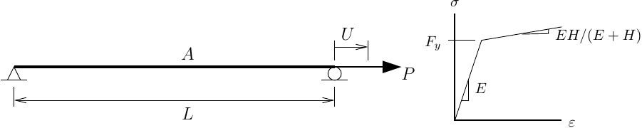
The definition of this model is straightforward. Mass is defined at the free DOF for dynamic analysis.

E = 29000
Fy = 50
Hkin = 500

A = 10
L = 100

g = 386.4
m = 1000/g

import openseespy.opensees as ops

ops.wipe()
ops.model('basic','-ndm',2,'-ndf',2)

ops.node(1,0,0); ops.fix(1,1,1)
ops.node(2,L,0); ops.fix(2,0,1)

ops.mass(2,m,0)

ops.uniaxialMaterial('Hardening',1,E,Fy,0,Hkin)

ops.element('truss',1,1,2,A,1)

The parameters for this model, i.e., the parameters with respect to which the response derivatives will be computed, are the material properties and the truss cross-section area.

ops.parameter(1,'element',1,'E')
ops.parameter(2,'element',1,'A')
ops.parameter(3,'element',1,'Fy')
ops.parameter(4,'element',1,'Hkin')

Three analyses are performed on the truss:

1. Load-control nonlinear static
2. Displacement-control nonlinear static
3. Nonlinear dynamic

For each analysis, the deterministic response is shown along with the derivative of the response with respect to each parameter listed above. Derivatives are scaled by the nominal parameter value so that the units match the original response.

Not shown here for brevity, the DDM derivatives have been verified against finite differences.

Load-Control Nonlinear Static Analysis

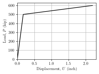
Ramping the applied load up to 1.2 times the yield load gives the load-displacement response shown below.

Useful commands in the script include getParamTags, which returns a list of all parameter tags defined for the model, and sensNodeDisp, which returns the nodal displacement sensitivity with respect to the specified parameter. Like reactions, OpenSees must be told when to compute the sensitivities via the sensitivityAlgorithm command with the -computeAtEachStep argument.

Py = A*Fy
Pmax = 1.2*Py
Nsteps = 100
dP = Pmax/Nsteps

ops.timeSeries('Linear',1)
ops.pattern('Plain',1,1)
ops.load(2,1.0,0)

ops.integrator('LoadControl',dP)
ops.analysis('Static')

ops.sensitivityAlgorithm('-computeAtEachStep')

for i in range(Nsteps):
    ops.analyze(1)
    print(ops.nodeDisp(2,1),ops.getLoadFactor())
    for param in ops.getParamTags():
        print(param,ops.sensNodeDisp(2,1,param))

For each parameter, the displacement sensitivity is plotted below on the x-axis while the y-axis is the applied load.

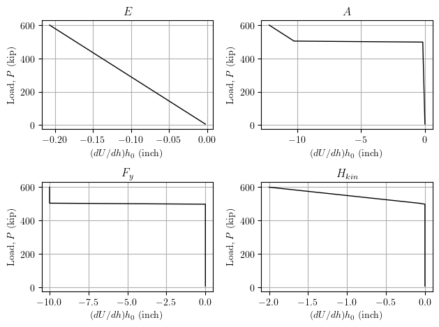
For each parameter, the displacement sensitivity is negative, i.e., the parameter acts as a “resistance” variable, where if the magnitude of the parameter increases, the magnitude of the displacement will decrease. Note that the displacement sensitivity with respect to the yield stress and the hardening modulus is zero prior to yield.

Displacement-Control Nonlinear Static Analysis

Instead of load control, performing displacement control on the free node gives the same load-displacement response as above.

The script for this analysis is shown below. Because the analysis is displacement controlled, we want to obtain the sensitivity of the load factor via the sensLambda command.

ops.timeSeries('Linear',1)
ops.pattern('Plain',1,1)
ops.load(2,1.0,0)

Umax = 2.2
Nsteps = 100
Uincr = Umax/Nsteps

ops.integrator('DisplacementControl',2,1,Uincr)
ops.analysis('Static')

ops.sensitivityAlgorithm('-computeAtEachStep')

for i in range(Nsteps):
    ops.analyze(1)
    print(ops.nodeDisp(2,1),ops.getLoadFactor(1))
    for param in ops.getParamTags():
        print(param,ops.sensLambda(1,param))

For each parameter, the load factor sensitivity is plotted below on the y-axis while the x-axis is the imposed displacement.

The positive load factor sensitivity indicates each parameter is a resistance variable, i.e., an increase in the parameter value will require more load to be applied in order to reach the imposed displacement. Again, the sensitivity with respect to yield stress and hardening modulus are zero prior to yield.

Nonlinear Dynamic Analysis

The DDM also works in dynamic analysis. Subjecting the truss model to uniform excitation and assigning 2% mass-proportional damping gives the displacement response history shown below.

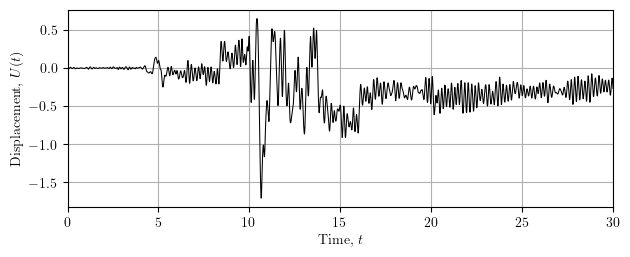
We can see there is permanent displacement, i.e., the material yields during the simulation and the sensitivities with respect to yield stress and hardening modulus parameters should be non-zero. The analysis script is shown below.

ops.timeSeries('Path',1,'-dt',0.02,'-filePath','tabasFN.txt')
ops.pattern('UniformExcitation',1,1,'-accel',1,'-factor',g)

dt = 0.005
Tmax = 30
Nsteps = int(Tmax/dt)

ops.integrator('Newmark',0.5,0.25)
ops.analysis('Transient')

ops.sensitivityAlgorithm('-computeAtEachStep')

for i in range(Nsteps):
    ops.analyze(1,dt)
    print(ops.getTime(),ops.nodeDisp(2,1))
    for param in ops.getParamTags():
        print(param,ops.sensNodeDisp(2,1,param))

The displacement response sensitivity with respect to each parameter is shown below.

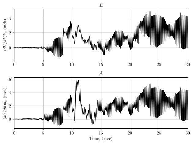
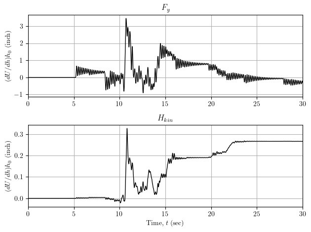
There’s a lot to imbibe in the plots of displacement response sensitivity: large oscillations in the sensitivity with respect to “elastic” parameters E and A and little bouts of damped free vibration in the sensitivity with respect to F_y and H_kin. I probably should have used a sine wave instead of a ground motion.

The DDM is not enabled for all element and material models in OpenSees, but it’s there for the basic element formulations like dispBeamColumn, forceBeamColumn, and a handful of solid elements, as well as fiber sections and materials like Hardening and Concrete01.